Analyze Respiratory Rate Variability (RRV)

Respiratory Rate Variability (RRV), or variations in respiratory rhythm, are crucial indices of general health and respiratory complications. This example shows how to use NeuroKit to perform RRV analysis.

Download Data and Extract Relevant Signals

# Load NeuroKit and other useful packages
import neurokit2 as nk
import numpy as np
import pandas as pd
import matplotlib.pyplot as plt
%matplotlib inline

plt.rcParams['figure.figsize'] = 15, 5  # Bigger images

In this example, we will download a dataset that contains electrocardiogram, respiratory, and electrodermal activity signals, and extract only the respiratory (RSP) signal.

# Get data
data = pd.read_csv("https://raw.githubusercontent.com/neuropsychology/NeuroKit/master/data/bio_eventrelated_100hz.csv")
rsp = data["RSP"]
nk.signal_plot(rsp, sampling_rate=100) # Visualize

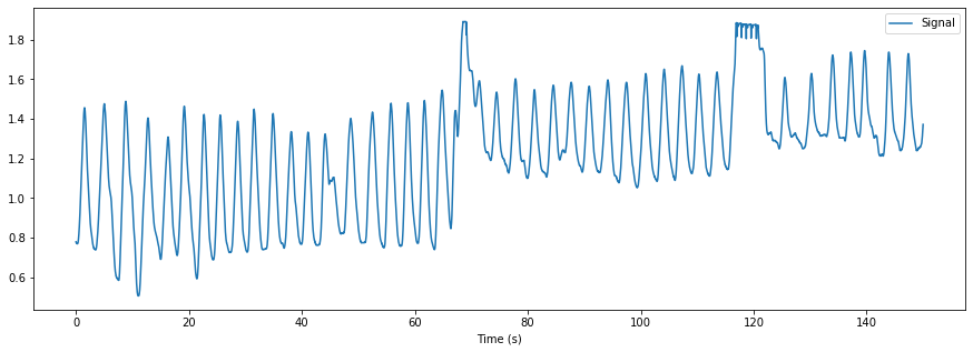
You now have the raw RSP signal in the shape of a vector (i.e., a one-dimensional array). You can then clean it using rsp_clean() and extract the inhalation peaks of the signal using rsp_peaks(). This will output 1) a dataframe indicating the occurrences of inhalation peaks and exhalation troughs (“1” marked in a list of zeros), and 2) a dictionary showing the samples of peaks and troughs.

Note: As the dataset has a frequency of 100Hz, make sure the ``sampling_rate`` is also set to 100Hz. It is critical that you specify the correct sampling rate of your signal throughout all the processing functions.

# Clean signal
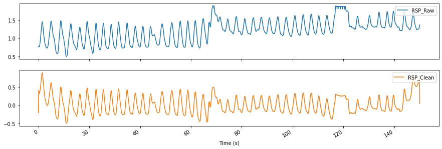
cleaned = nk.rsp_clean(rsp, sampling_rate=100)

# Extract peaks
df, peaks_dict = nk.rsp_peaks(cleaned)
info = nk.rsp_fixpeaks(peaks_dict)
formatted = nk.signal_formatpeaks(info, desired_length=len(cleaned),peak_indices=info["RSP_Peaks"])

nk.signal_plot(pd.DataFrame({"RSP_Raw": rsp, "RSP_Clean": cleaned}), sampling_rate=100, subplots=True)

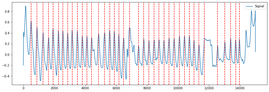
candidate_peaks = nk.events_plot(peaks_dict['RSP_Peaks'], cleaned)

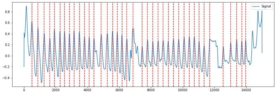
fixed_peaks = nk.events_plot(info['RSP_Peaks'], cleaned)

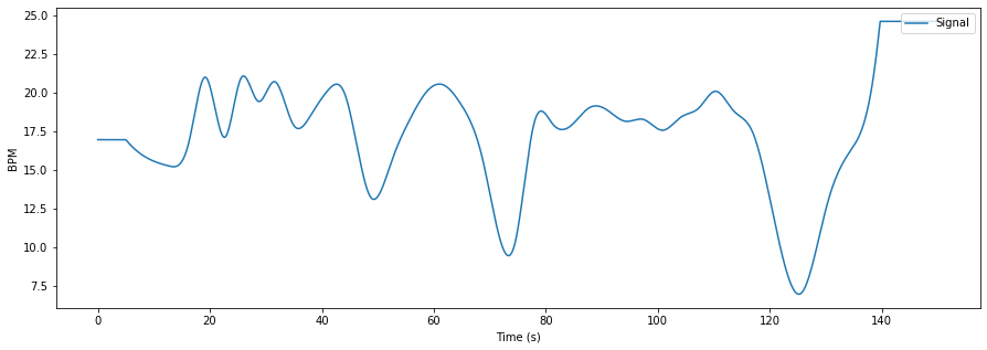
# Extract rate
rsp_rate = nk.rsp_rate(formatted, desired_length=None, sampling_rate=100) # Note: You can also replace info with peaks dictionary

# Visualize
nk.signal_plot(rsp_rate, sampling_rate=100)
plt.ylabel('BPM')

Text(0, 0.5, 'BPM')

Analyse RRV

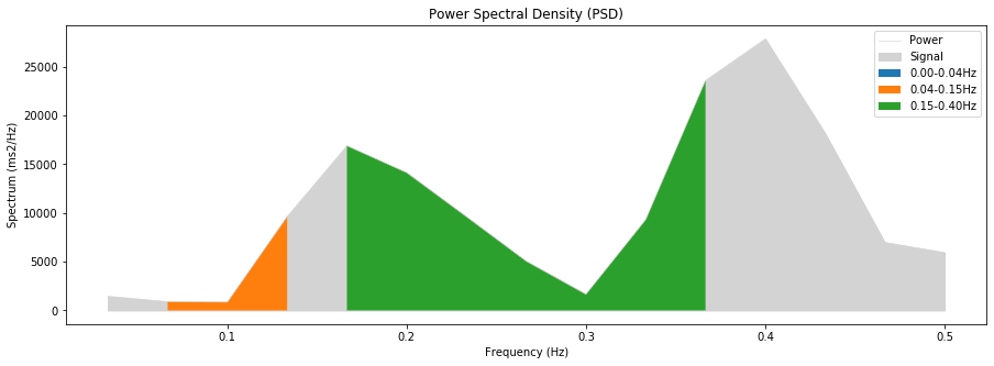
Now that we have extracted the respiratory rate signal and the peaks dictionary, you can then input these into rsp_rrv(). This outputs a variety of RRV indices including time domain, frequency domain, and nonlinear features. Examples of time domain features include RMSSD (root-mean-squared standard deviation) or SDBB (standard deviation of the breath-to-breath intervals). Power spectral analyses (e.g., LF, HF, LFHF) and entropy measures (e.g., sample entropy, SampEn where smaller values indicate that respiratory rate is regular and predictable) are also examples of frequency domain and nonlinear features respectively.

A Poincaré plot is also shown when setting show=True, plotting each breath-to-breath interval against the next successive one. It shows the distribution of successive respiratory rates.

rrv = nk.rsp_rrv(rsp_rate, info, sampling_rate=100, show=True)
rrv

Neurokit warning: signal_psd(): The duration of recording is too short to support a sufficiently long window for high frequency resolution. Consider using a longer recording or increasing the `min_frequency`

	RRV_SDBB	RRV_RMSSD	RRV_SDSD	RRV_VLF	RRV_LF	RRV_HF	RRV_LFHF	RRV_LFn	RRV_HFn	RRV_SD1	RRV_SD2	RRV_SD2SD1	RRV_ApEn	RRV_SampEn	RRV_DFA
0	1030.411296	1269.625397	1286.590811	0.0	203.846501	2000.465169	0.1019	0.092476	0.907524	909.757087	1138.34833	1.251266	0.496939	0.693147	0.755783

This is a simple visualization tool for short-term (SD1) and long-term variability (SD2) in respiratory rhythm.

See documentation for full reference

RRV method taken from : Soni et al. 2019